Visualization of Multivariate Data
Using 3D and VR Presentations
Vladimir Batagelj
University of Ljubljana, Faculty of mathematics and physics
Department of Mathematics, Jadranska 19, 1000 Ljubljana
Tel: 386 (61) 1766 672; fax: 386 (61) 217 281
e-mail:
Vladimir.Batagelj@uni-lj.si
WWW:
http://vlado.fmf.uni-lj.si/
Andrej Mrvar
University of Ljubljana, Faculty of Social Sciences
Kardeljeva pl. 5, 1000 Ljubljana
e-mail:
Andrej.Mrvar@uni-lj.si
WWW:
http://www.uni-lj.si/~fdmrvar/andrej.html
Abstract
VRML (Virtual Reality Modeling Language) and freely available browsers for
it made three dimensional presentations very popular also on
personal computers.
One of the most important features of VRML is the possibility of
traveling in the obtained scene - egocentric view.
In the paper an introduction to visualization of multivariate
data and some examples of their VR presentations are given.
Paper published in: Indo-French Workshop on Symbolic Data Analysis
and its Applications. 23-25. September 1997, Paris XI - Dauphine,
vol 1., p. 66-76.
1. Introduction
1.1 Data Visualization
With the growth of computing power of desktop computers, data
visualization is gaining popularity among researchers as
a tool for data exploring and for
presentations of results (Brown 95,
Baker 95.)
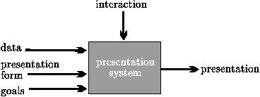
Using a data visualization system (see Figure 1) a researcher
usually adopts different goals (Wahrend 90) to:
identify, locate, distinguish, categorize,
cluster, rank, compare, associate or correlate some data.
Figure 1. Data visualization system.
|
Properties of the data set that crucially influence
forms of its representation are:
- size: small, large, infinite;
- density: sparse, dense, cluttered; and
- activity: static, dynamic (deterministic, random).
Small data sets can be presented in totality and in
detail in a single view. In an overall view of large
data sets details are lost; and a detailed view can
encompass only a part of data set.
The basic feature of VR (Virtual Reality) is the support of
egocentric view -
the user is immersed into the presentation as its active part;
he can travel inside the data scene, the view
is determined by his position in the scene.
Standard data visualizations supported by general
purpose programs (Excel, PowerPoint, ...) are mostly
exocentric - viewer is positioned outside
the presentation. Often the third dimension is used
only to make the presentation fancier, and not to get
better insight about the data.
In very large data sets a serious problem appears:
How to avoid to be ``lost within the forest''?
There are several solutions that help the
user's orientation:
- restart option: returns the user to the
starting position;
- introduction of additional orientation elements:
coordinates display, grids, shadows, landmarks
(static / user set). These elements can be switched
on/off.
- multiview: consists of at least two views
(windows):
- map view: overall view (usually exocentric)
which contains the current position and allows
'long' moves (jumps). For very large data sets
it can be combined with zooming or fish eye.
- local view: which displays the selected
portion of data set.
Additional support can be achieved by implementing
trace/backtrack/replay mechanism and
guided tours.
Closely related with the multiview idea are the concepts of
glasses, lenses and
zooming (
Pad++,
inXight 96).
Selecting different glasses we obtain different views on the same data.
Glasses have effect on the entire window, and lenses only on the
selected region.
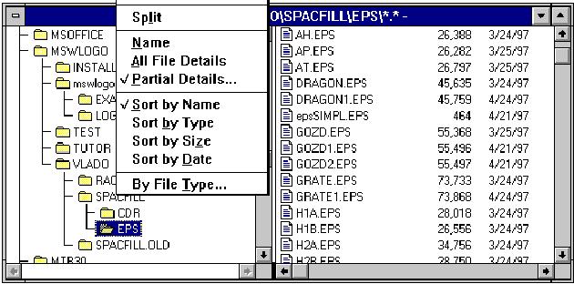
Figure 2. Windows File Manager.
|
An example of the multiview approach is the presentation of
files used in windows file manager (see Figure 2).
It provides also different glasses (Name, All File Details, ...,
Sort by ...; in the new version: Large icons, Small icons,
List, Detailed list, ...).
1.2 Visualization of Multivariate Data Sets
In visualizing multivariate data we usually
deal with small or large, sparse and static data sets.
Let E = Xi be a set of units.
A unit X is usually described by list of values
of selected attributes (properties)
(V1=x1,V2=x2,...,Vm=xm).
It is usually represented by a glyph which integrates,
as its components, elements representing unit's attributes.
From standard data analysis we know several types of
2D-glyphs: point in plane, pie charts, bar charts, columns, stars,
Chernoff faces, Andrews curves, ... (Dillon 84).
Most of 2D-glyphs can be extended to 3D-glyphs, and
some additional should be invented.
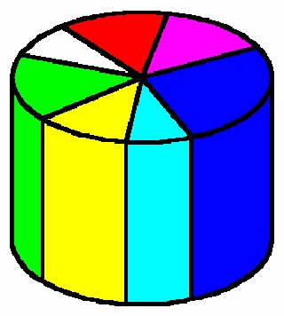
For example, pie chart and column representation can be combined
into pie cylinder (see Figure 3).
By using these glyphs to represent representatives
(centroids) of groups, they can be used also for
presentations of groups.
Figure 3. Pie Cylinder.
|
For representing selected attribute over a group of
units histograms and Tukey's box-and-whisker plots are often used
(see Figure 4).
Figure 4. Tukey Glyph.
|
They can be combined into a glyph (for example, a star)
representing a group (see picture in subsection 2.2 Stars)
The largest ring in Tukey glyph represents
data set (population) average, the middle ring - group average,
and the small one - group median. The tubes are representing
1-3 quartile, 1-9 decile and min-max intervals.
The representation elements support associative,
selective, ordering and/or quantifying tasks.
In the visualization task there are several levels of
detail represented by the hierarchy
(attribute, unit, group, groups, data set)
Most of data analysis procedures can be seen as
transformations on or relations between these
levels.
Different scale types are represented by different
graphical elements:
| scale | representation
|
| nominal | color, shape
|
| ordinal | grade, lightness, texture, arrangement (position)
|
| numeric | size, position, direction, angle
|
Since
numeric is included in ordinal,
and ordinal is included in nominal,
the representations compatible with higher scales
could be used also for lower scales - e.g.,
direction to represent nationality. A general rule is
that this should be avoided because they can suggest
unsubstantial associations.
1.3 Three Dimensional Data Presentations
In this paper we discuss 3D presentations of multivariate data.
As a prototyping environment we selected VRML
(Virtual Reality Modeling Language) because it provides a
platform independent presentations and supports VR presentations.
Figure 5. Basic VRML Shapes.
|
In a presentation of multivariate data several VRML elements
can be used:
- position in space (x, y, z);
- shape (sphere, cube, cone, cylinder, plane, ...;
see Figure 5);
- color;
- size, angle, slope, area, volume;
- pattern (texture);
- direction (orientation);
- text;
- lights (different light sources, shadowing,
transparency, reflections, ...);
- rotation of objects;
- different views and ways of moving in the obtained scene;
camera properties
(orthographic, perspective, stereoscopic; field of view).
1.4 VRML
During the first Web Conference in May 1994 some experts for virtual
reality formed a group that should prepare some additions to HTML
(HyperText Markup Language) in the field of virtual reality.
So the idea of VRML (Virtual Reality Markup Language) was born.
Silicon Graphics supported the idea significantly by
giving in free use its language for description of three dimensional
objects Open Inventor (Warnecke 94) together with its parser.
On the next conference, in October 1994 in Chicago, first version of
VRML was announced
(
Bell, Ames 96).
Designers decided that HTML and VRML should be
"orthogonal" but connected languages - VRML became
Virtual Reality Modeling Language.
First shareware VRML browser WebSpace appeared in May 1995.
Paper company gave the browser WebFX
in free use in August 1995. WebFX was a plug-in for Netscape
- the most popular HTML browser at that time.
WebFX was later renamed to live3D. Silicon Graphics
is developing its own VRML viewer -
CosmoPlayer.
At Siggraph (August 1996) the VRML 2.0 specification was published
and made available in its final form (Lea 96).
VRML 2.0 allows the user to build user controlled multiuser scenes.
VRML is used in many areas: data organization, three dimensional maps,
modeling, mathematics, chemistry, medicine,...
(
Vollhardt).
2. Examples
In the following examples data about 27 different types of food
are used (see table; Hart 75).
They are described by 5 numeric variables:
Food Energy, Protein, Fat, Calcium, and Iron.
Variables were standardized before use.
Table 1. Types of Food (Raw Data).
| No | Food | Cluster | Energy (cal) | Protein (g) | Fat (g) | Calcium (mg) | Iron (mg)
|
| 1 | Beef, braised | 3 | 340 | 20 | 28 | 9 | 2.6
|
| 2 | Hamburger | 3 | 245 | 21 | 17 | 9 | 2.7
|
| 3 | Beef, roast | 3 | 420 | 15 | 39 | 7 | 2.0
|
| 4 | Beef, steak | 3 | 375 | 19 | 32 | 9 | 2.6
|
| 5 | Beef, canned | 3 | 180 | 22 | 10 | 17 | 3.7
|
| 6 | Chicken, broiled | 6 | 115 | 20 | 3 | 8 | 1.4
|
| 7 | Chicken, canned | 6 | 170 | 25 | 7 | 12 | 1.5
|
| 8 | Beef heart | 3 | 160 | 26 | 5 | 14 | 5.9
|
| 9 | Lamb leg, roast | 5 | 265 | 20 | 20 | 9 | 2.6
|
| 10 | Lamb shoulder, roast | 5 | 300 | 18 | 25 | 9 | 2.3
|
| 11 | Smoked ham | 4 | 340 | 20 | 28 | 9 | 2.5
|
| 12 | Pork, roast | 4 | 340 | 19 | 29 | 9 | 2.5
|
| 13 | Pork, simmered | 4 | 355 | 19 | 30 | 9 | 2.4
|
| 14 | Beef tongue | 3 | 205 | 18 | 14 | 7 | 2.5
|
| 15 | Veal cutlet | 3 | 185 | 23 | 9 | 9 | 2.7
|
| 16 | Bluefish, baked | 2 | 135 | 22 | 4 | 25 | 0.6
|
| 17 | Clams, raw | 1 | 70 | 11 | 1 | 82 | 6.0
|
| 18 | Clams, canned | 1 | 45 | 7 | 1 | 74 | 5.4
|
| 19 | Crabmeat, canned | 1 | 90 | 14 | 2 | 38 | 0.8
|
| 20 | Haddock, fried | 2 | 135 | 16 | 5 | 15 | 0.5
|
| 21 | Mackerel, broiled | 2 | 200 | 19 | 13 | 5 | 1.0
|
| 22 | Mackerel, canned | 2 | 155 | 16 | 9 | 157 | 1.8
|
| 23 | Perch, fried | 2 | 195 | 16 | 11 | 14 | 1.3
|
| 24 | Salmon, canned | 2 | 120 | 17 | 5 | 159 | 0.7
|
| 25 | Sardines, canned | 2 | 180 | 22 | 9 | 367 | 2.5
|
| 26 | Tuna, canned | 2 | 170 | 25 | 7 | 7 | 1.2
|
| 27 | Shrimp, canned | 1 | 110 | 23 | 1 | 98 | 2.6
|
Units (types of food) were manually clustered in six clusters,
represented by colors
- clams and crabs / cyan,
- fish / blue,
- beef / magenta,
- pork / red,
- lamb / yellow,
- chicken / white.
The two main clusters
- {1, 2} - sea-food, and
- {3, 4, 5, 6} - meat
are represented by shape (cube, sphere).
Since the full advantage of VRML can be grasped only using
VRML browser we strongly recommend the reader to visit the
HTML/VRML version of this paper at:
http://vlado.fmf.uni-lj.si/vrml/paris.97/
Software for producing 3D representations of multivariate
data in VRML is available at:
http://vlado.fmf.uni-lj.si/pub/vrml/
2.1 Planets
The simplest presentation of multivariate data is a presentation
using planets: three selected variables are shown
using positions in the space. Additional information can be represented
by glyphs that represent units.
In presentation of food types in Figure 6 the positions
in the space are determined by first three principal components.
Different views can show interesting relations in data.
For example, the positions of glyphs representing clams and crabs
suggest that our decision to put them in the same group was
not appropriate. Groups of similar types of food can be easily
noticed in both pictures.
Planets (VRML)
Figure 6. Planets.
|
2.2 Stars
The use of stars is an alternative possibility to present
multivariate data. Each variable is represented using the length
of the corresponding ray of the star. We can also use different
colors for different rays.
In Figure 7 positions in the space are again determined
by the first three principal components. If we look at the pictures
we can see that the shapes of the stars explain their positions in
the space (or vice versa) - stars that are closer are more similar
than the others.
Stars (VRML)
Figure 7. Stars.
|
In Figure 8 the two main clusters
(sea-food - left side, meat - right side)
are represented using Tukey stars.
We can easily see main differences between them -
low level and small variation of Fat and Energy in fish cluster,
and of Calcium in meat cluster.
Tukey stars can be, by introducing appropriate glyphs,
used also for representing groups of units described
by all three types of variables (nominal, ordinal, numeric).
Fish (VRML)
Meat (VRML)
Figure 8. Tukey Stars.
|
2.3 3D Histograms
We can represent multivariate data also using 3D histograms.
In presentation in Figure 9 the first two principal
components determine the positions in the plane (value 0);
the standardized variable Fat determines the height of corresponding
column; six clusters are represented by color, and the main
two clusters by shape of the column (prism, cylinder).
3D Histogram (VRML)
Figure 9. 3D Histogram.

|
2.4 3D Dendrograms
Hierarchical clustering is often used in data analysis.
The process of fusing can be shown using dendrograms.
We can combine this method with principal components.
The first two principal components determine the position of a unit
in the plane. Units are then joined using 3D dendrogram according
to hierarchical clustering algorithm.
In this way we can find some similarities between the results of
both methods (see Figure 10):
units that are closer (according to principal components) are joined
earlier than the others.
3D Dendrogram (VRML)
Figure 10. 3D Dendrogram.

|
2.5 3D Time Series Spiral
In Figure 11 quarterly, seasonally unadjusted time series at
1964 prices Private consumer expenditure in Austria
(billions of Austrian Schillings) (Thury 82) is represented by
time series spiral.
In January 1978 a special purchase tax rate for luxury goods was
to be introduced. Therefore, most consumers bought the durable
goods, and above all cars, which they intended to purchase in the
immediate future, at the end of 1977.
3D Time Series Spiral (VRML)
Figure 11. 3D Time Series Spiral.
|
3. Conclusion
In the paper we presented some general ideas on data visualization
and some examples of visualization of multivariate data.
On this basis different kinds of programs for multivariate data
visualization can be developed - from simple transformers of
multivariate data to their VRML descriptions, to a visual data
exploration system, based on some powerful 3D-graphic library
(OpenGL, Direct3D, ...), combined with other data analysis
methods.
References
-
Ames A.L., Nadeau D.R., Moreland J.L.:
The VRML Sourcebook.
Wiley, New York, 1996.
-
Baker M.P., Wickens C.D.:
Human Factors in Virtual Environments for
the Visual Analysis of Scientific Data.
draft, 1995.
http://monet.ncsa.uiuc.edu/~baker/PNL/paper.html
-
Batagelj V., Mrvar A.:
Trirazsezne predstavitve podatkov (3D Data Presentations).
Proceedings of DSI'96, Portoroz, April 17-24, 1996, p. 427-432.
-
Bell G., Parisi A., Pesce M.:
The Virtual Reality Modeling Language.
Version 1.0 Specification.
http://www.sdsc.edu/vrml_repository/Archives/vrml10-3.html
-
Brown J.R., Earnshaw R., Jern M., Vince J.:
Visualization: Using Computer to Explore Data and Present
Information. Wiley, New York, 1995.
-
Dillon W.R., Goldstein M.:
Multivariate Analysis: Methods and Applications.
Wiley, New York, 1984, p. 191-202.
-
Hartigan J.A.:
Clustering Algorithms.
Wiley, New York, 1975, p.86.
-
inXight:
VizControls Technology.
A Xerox New Enterprise Company, 1996.
http://www.inxight.com/products/visual/overview.shtml
-
Lea R., Matsuda K., Miyashita K.:
Java for 3D and VRML Worlds.
New Riders, Indianapolis, 1996.
-
Pad++:
Portal filtering and 'magic lenses'.
http://www.cs.unm.edu/pad++/lenses.html
-
Thury G.:
Modelling Consumer Expenditure by Intervention Analysis.
TIME SERIES: Theory and Practice 1; O.D. Anderson (editor).
North Holland, 1982, p. 308.
-
Tukey J.W.:
Exploratory Data Analysis.
Addison-Wesley, Reading, MA, 1977.
-
VRML in Chemistry:
Vollhardt H., Moeckel G., Henn C., Teschner M., and Brickmann J.:
VRML for the Communication with 3D Scenarios of Biomolecules.
http://ws05.pc.chemie.th-darmstadt.de/vrmlG/
-
Warnecke J.:
The Inventor Mentor.
Addison-Wesley, Reading, MA, 1994.
-
Wehrend S., Lewis C.:
A Problem-Oriented Classification of Visualization
techniques. In Proceedings of IEEE Visualization'90, 1990,
p. 139-143.
-
Young F.W., Edds T., Kent D., Kuhfeld W.F.:
Visual Exploratory Data Analysis.
In: Classification as a Tool of Research, Proceedings of the 9th
Annual Meeting of the Classification Society (F.R.G),
University of Karlsruhe, F.R.G., 26-28 June, 1985.
edited by W. Gaul and M. Schader.